@katiejolly6
on
Writing a classification algorithm to build precinct shapefiles in Ohio
About the project
This past summer I worked at the Voting Rights Data Institute at Tufts and MIT in Cambridge, MA. Broadly, we worked on projects related to the mathematical and computational aspects of gerrymandering research. My main project was creating an open source precinct shapefile for Ohio. We started with a list of 88 county names and over the summer built a full shapefile and joined it to as many statewide election returns as possible since 2010. In the process I gained an appreciation for county government employees, Twitter as an academic resource, and crowdsourcing data collection.
Precincts are the smallest unit at which election data in the United States are reported. In order to make nuanced arguments about the fairness of districts, we need to know about the precinct boundaries. Recently in the news, with the election and decennial census approaching in 2020, there has been a resurgent interest in polling place accessibility, voter registration campaigns, and (sometimes hidden) voter disenfranchisement. For example, there’s an ACLU lawsuit in Georgia now over closing polling places in predominantly African-American areas. The Supreme Court also recently upheld Ohio’s practice of purging inactive voters from the voter rolls. Many of the most pressing voting rights challenges require precise knowledge of where polling places are and who is using those polling places, as well as which voters are affected by new policies.
This project aims to make it easier for community members to learn more about their own precincts and create one way for people to support concerns about equity and fairness with numbers. We focus on Ohio, but we hope our methodology can be repeated in other states as well and support the work of groups working on similar research.
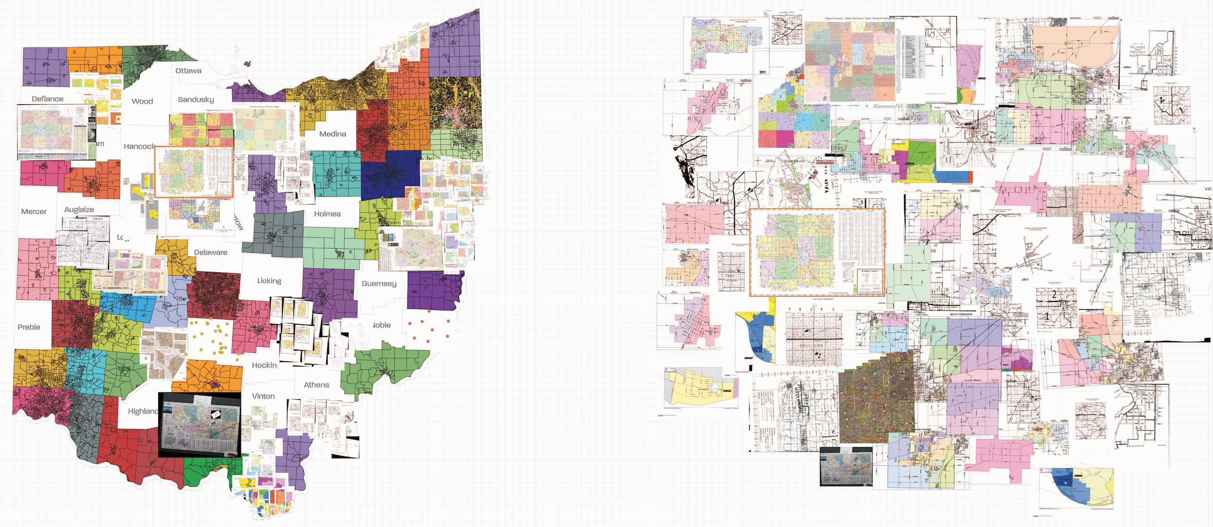
In June we started with a list of the 88 counties in Ohio. For each county we looked online for a publicly available shapefile. Most counties did not have one, though. For counties that were missing some piece of information (shapefile, date of adoption, etc.) we called the Board of Elections or GIS office. Still many counties did not have a shapefile, but they were often able to provide a PDF or paper map through the mail. In total, we were given shapefiles from 50 counties, PDF or paper maps from 31 counties, and no maps from 7 counties.
In this post I’ll discuss how we approximated precinct boundaries for those counties that didn’t have any maps. There are a variety of ways to do this and we chose the one we could do in the amount of time we had given our resources.

What to do when there’s no map?
“Geocoding is the process of transforming a description of a location—such as a pair of coordinates, an address, or a name of a place—to a location on the earth’s surface.” Commonly geocoding an address returns latitude/longitude coordinates so that you can use that address for spatial analysis. Many projects that try to build precinct boundaries from voter addresses use this kind of geocoding. Ultimately, we wanted to try something different.
Instead of returning latitude/longitude coordinates, we used a Census API through the tigris package that returns the GEOid of the census block of the address. This provides slightly less precise information but it tends to have higher accuracy, as measured by the number of addresses that return an NA for either method given that we started with the same set of addresses. A geocoding service like Google Maps also works, but it’s strictly rate-limited at 2,500 requests per day. Even the smallest counties in Ohio have far more than 2,500 registered voters.
Geocoding is important for this project because it is essentially how we will translate the voter registration addresses to a general precinct outline. We then use an algorithm to draw more concrete lines around voters.
The algorithm
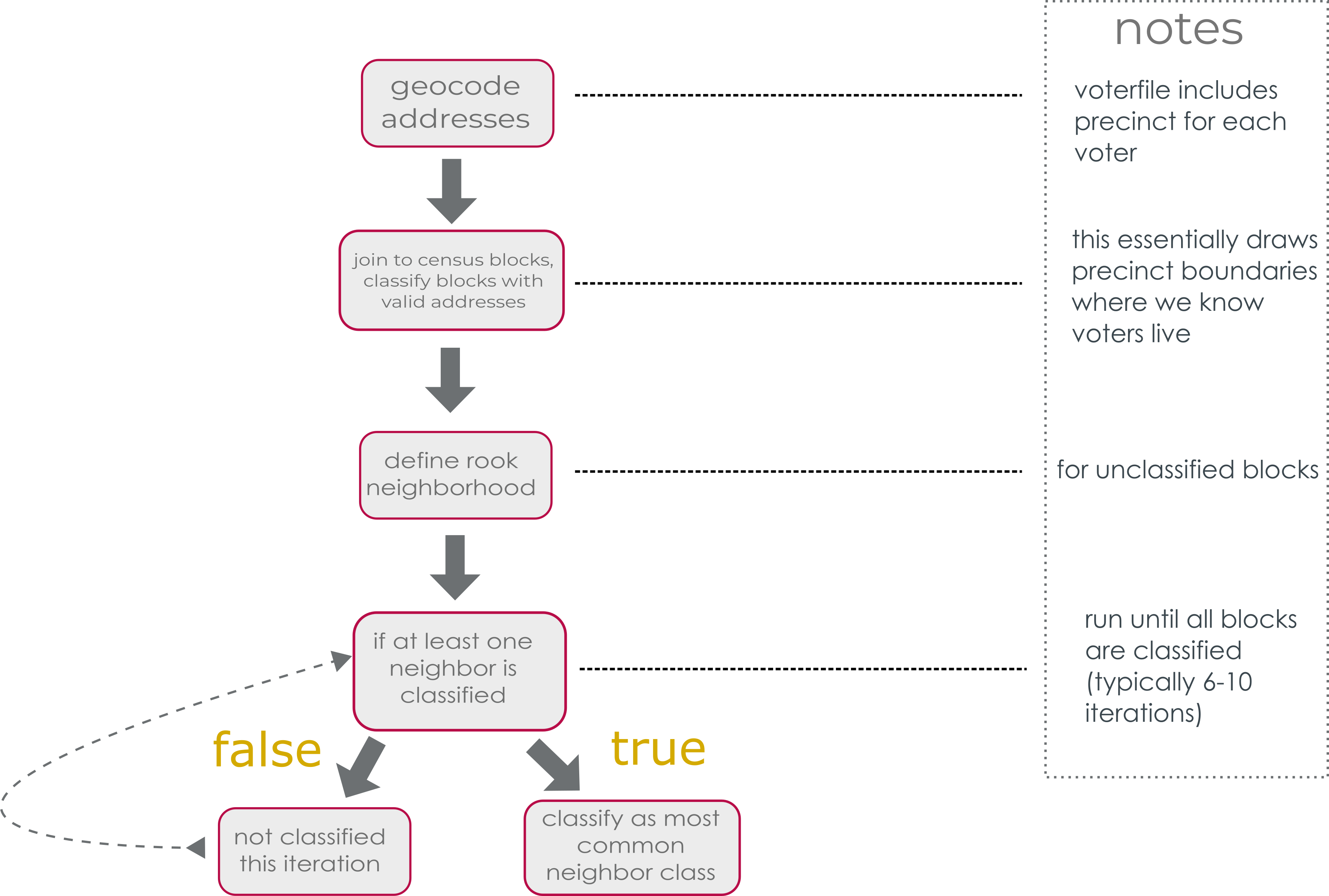
In broad strokes, our algorithm takes the geocoded addresses (with the information about what precinct the voter is assigned to) and assigns precinct boundaries by census block. So it finds the blocks that already have valid addresses, usually 40-60% of the blocks, and assigns it to the most common precinct designation of the voters. Then for the unclassified blocks, we classify them based on their rook-contiguity neighbors. I’ll illustrate this process using Noble County as an example below.

Step 1: Getting the block IDs
We can get the voterfile for any county in Ohio from the Secretary of State website.
This includes voter data such as name, addresses, and precinct.
library(tidyverse)
library(tigris)
library(sf)
library(magick)

noble <- read_csv("https://www6.sos.state.oh.us/ords/f?p=VOTERFTP:DOWNLOAD::FILE:NO:2:P2_PRODUCT_NUMBER:61") # download the voterfile for Noble County
| SOS_VOTERID | PARTY_AFFILIATION | RESIDENTIAL_ADDRESS1 | RESIDENTIAL_CITY | RESIDENTIAL_STATE | VOTER_STATUS |
|---|---|---|---|---|---|
| OH0012094732 | NA | 44759 BUCKEYE DR | CALDWELL | OH | ACTIVE |
| OH0012090545 | D | 48840 HILLCREST LN | CALDWELL | OH | ACTIVE |
| OH0022355950 | D | 19052 WOODSFIELD RD | CALDWELL | OH | ACTIVE |
| OH0012088260 | NA | 41475 PARKS HILL RD | CALDWELL | OH | ACTIVE |
| OH0022580793 | D | 14194 CROOKED TREE RD | LOWELL | OH | ACTIVE |
| OH0012086321 | R | 48386 SENECA LAKE RD | SARAHSVILLE | OH | ACTIVE |
We can then geocode the addresses in the voterfile. This code gets the census block GEOid for each address. This will allow us to classify census blocks to precinct when they have a registered voter there.
noble$GEOID10 <- NA # initialize an empty column

# the call geolocator function takes the address, city, and state as individual columns and sends them as a request to the census bureau API

vec <- purrr::map_chr(1:nrow(noble), function(i) tigris::call_geolocator(noble[['RESIDENTIAL_ADDRESS1']][i],
                                                                         noble[['RESIDENTIAL_CITY']][i],
                                                                         noble[['RESIDENTIAL_STATE']][i]))
Once we have those GEOids, we can run our classification algorithm to approximate the precinct of census blocks without registered voters.
Step 2: Classification algorithm
The general structure of our algorithm is diagrammed below. Essentially we geocode the addresses, classify blocks with voters in them, then use rook neighbors to classify any unclassified blocks.

Below are the functions we’ll need for the main classification algorithm.
# helper functions

st_rook = function(a, b = a) sf::st_relate(a, b, pattern = "F***1****") # find rook-contiguity neighbors

lookup_precinct <- function(index, precinct_name_var = "PRECINCT_NAME"){ # for a given row index, find the precinct name
  precinct <- precincts_nb[index, precinct_name_var]
  return(precinct)
}

create_precinct_vector <- function(){ # create a vector of precinct names from lookup_precinct
  prec <- purrr::map(precincts_nb$NB_ROOK, lookup_precinct)
  prec_vec <- purrr::map(prec, dplyr::pull)
  return(prec_vec)
}


clean_precincts_fun <- function(i){ # clean the precincts, take out NA values
  y <- precincts_nb_sub$precinct_nn[[i]]
  print(y)
  new_y <- y[!is.na(y)]
  return(new_y)
}
#################################################

# Use this function to assign 2010 census blocks to a particular precinct based on the most common precinct assignment of the voters geotagged there.

join_voters_to_blocks <- function(voters, blocks, block_geoid_voters = "BLOCK_GEOID", precinct_name = "PRECINCT_NAME"){
  colnames(voters)[colnames(voters)==block_geoid_voters] <- 'BLOCK_GEOID'
  colnames(voters)[colnames(voters)==precinct_name] <- 'PRECINCT_NAME'
  precincts <- voters %>%
    # mutate(BLOCK_GEOID = as.character(!! block_geoid_q)) %>%
    # rename(PRECINCT_NAME = (!! precinct_name_q)) %>%
    dplyr::group_by(BLOCK_GEOID, PRECINCT_NAME) %>% # for each block, precinct combination
    dplyr::summarise(c=n()) %>% # counts the number of times a precinct is counted for a particular block
    dplyr::filter(row_number(desc(c))==1) # dataframe of precincts from voterfile, takes the most common precinct assignment for a block

  precincts_geo <- blocks %>%
    dplyr::mutate(GEOID10 = (GEOID10)) %>%
    dplyr::left_join(precincts, by = c("GEOID10" = "BLOCK_GEOID")) %>% # combine precincts with block shapefile
    dplyr::mutate(dimension = st_dimension(.)) %>%
    dplyr::filter(!(is.na(dimension))) # take out empty polygons

  return(precincts_geo)

}

# Assign a neighborhood to each block

find_neighbors <- function(x, type = "rook"){
  if (type == "rook"){
    NB <- st_rook(x)
  } else if (type == "queen") {
    NB <- st_queen(x)
  } else {
    stop("Please enter 'rook' or 'queen' for neighbor type")
  }
  x$NB <- NA
  for (i in 1:length(NB)){
    x$NB[i] <- NB[i]
  }

  return(x)
}

# Lookup the precinct names of each block in a neighborhood.


lookup_precincts_nn <- function(x){
  precinct_nn <- list()

  for (i in 1:nrow(x)) {
    precincts <- c()

    for (y in x$NB[[i]]){
      precincts <- c(precincts, x[[y, 'PRECINCT_NAME']])
    }

    precinct_nn[[i]] <- precincts

  }

  x$precinct_nn <- precinct_nn

  return(x)

}

# Classify any unassigned block with the most common precinct name of the rook-neighborhood.

classify_nn <- function(x){
  precincts_nb_sub <- x %>%
    filter(!is.na(precinct_nn),
           !identical(precinct_nn, character(0)))

  clean_precincts_fun <- function(i){
    y <- precincts_nb_sub$precinct_nn[[i]]
    new_y <- y[!is.na(y)]
    return(new_y)
  }

  p_new <- map(1:nrow(precincts_nb_sub), clean_precincts_fun)

  p_lengths <- map(1:length(p_new), function(x) length(p_new[[x]]))

  precincts_nb_sub <- precincts_nb_sub %>%
    mutate(precinct_nn_clean = p_new,
           precinct_nn_length = p_lengths) %>%
    filter(precinct_nn_length > 0) # take out the blocks without meaningful neighbors

  for (i in 1:nrow(precincts_nb_sub)){
    precincts_nb_sub$PRECINCT_NAME[i] <- ifelse(is.na(precincts_nb_sub$PRECINCT_NAME[i]), names(which.max(table(precincts_nb_sub$precinct_nn[[i]]))), precincts_nb_sub$PRECINCT_NAME[i])
  } # assign a precinct as the max of the vector of precincts

  precincts_nb_full <- x %>%
    left_join(precincts_nb_sub %>% st_set_geometry(NULL) %>% select(GEOID10, PRECINCT_NAME), by = "GEOID10") %>%
    mutate(PRECINCT_NAME.x = if_else(is.na(PRECINCT_NAME.x), PRECINCT_NAME.y, PRECINCT_NAME.x)) %>%
    select(-PRECINCT_NAME.y) %>%
    rename(PRECINCT_NAME = PRECINCT_NAME.x)

  message(paste0("There are ", sum(is.na(x$PRECINCT_NAME)), " unclassified blocks."))

  return(precincts_nb_full)
}
Now that we have functions, we can chain them all together with %>% for readability.
Classifying precincts in Noble County
blocks <- tigris::blocks(state = "OH", county = "Noble")

blocks_sf <- blocks %>%
  st_as_sf()
# first iteration

noble_nn1 <- noble %>%
  mutate(BLOCK_GEOID = as.character(BLOCK_GEOID)) %>%
  join_voters_to_blocks(blocks_sf) %>%
  find_neighbors() %>%
  lookup_precincts_nn() %>%
  classify_nn()
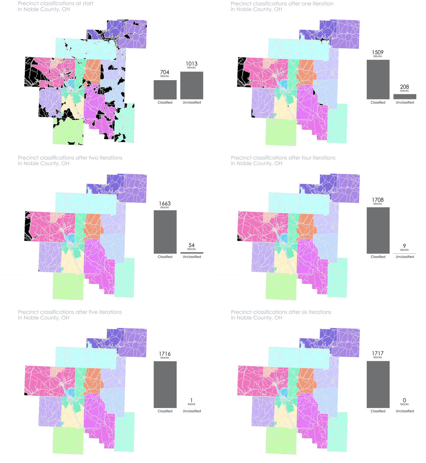
With the built-in message, we know that there are 1,013 blocks left to classify. We run through this algorithm again to classify more of those blocks.
noble_nn2 <- noble_nn1 %>% # start with what is already classified
  lookup_precincts_nn() %>% # we don't need to find the list of neighbors again, just update their assigned precincts
  classify_nn()
After this second iteration we only have 208 unclassified blocks. We continue this pattern until we get the message that there are 0 more unclassified blocks
noble_nn3 <- noble_nn2 %>%
  lookup_precincts_nn() %>%
  classify_nn()

noble_nn4 <- noble_nn3 %>%
  lookup_precincts_nn() %>%
  classify_nn()

noble_nn5 <- noble_nn4 %>%
  lookup_precincts_nn() %>%
  classify_nn()

noble_nn6 <- noble_nn5 %>%
  lookup_precincts_nn() %>%
  classify_nn()

noble_nn7 <- noble_nn6 %>%
  lookup_precincts_nn() %>%
  classify_nn()
After several iterations we have 0 unclassified blocks.
I’ve created an animation below that details visually how the algorithm works. You can follow along with the bars to see how many unclassified blocks remain after each run.

At this point we’ve created our precinct shapefile! We can dissolve on the PRECINCT_NAME field to get single polygons for each one, instead of having them as blocks.
In order to use these shapefiles we want to have some idea of how accurate they actually are. It’s hard to evaluate for the counties that didn’t provide us with “true” values, or actual precinct boundaries. Instead we can measure our accuracy using other counties that we do have “true” values for and then apply what we learn back to counties like Noble. That process is longer than what I’ll include in this post, so check back later for that!
In the next post I will discuss how we evaluate these shapefiles using the spatial v-measure from the sabre package (and inspired by this blog post).