Evaluating our precinct boundary approximation algorithm with v-measure

Introduction and intuition

In the last post, I described the algorithm we wrote to approximate precinct boundaries in Ohio. We were pretty happy with how it was performing based on common sense, but wanted a way to quantify the error. One problem we ran into was that we did not have a good way to verify the accuracy of precinct boundaries in counties that did not have maps. Instead, we used counties that did provide maps to verify accuracy broadly. We essentially treated them as “no maps” for approximation purposes so we could see how close our algorithm was. In the actual shapefile, though, we used the maps provided by the county.

We tried a few different ways to calculate error in our algorithm. One way that we used for a while was to find the percent of the total area in a county that was mis-assigned. This worked, but it didn’t really tell us all that much useful information about where the errors were occurring most often in the county. It only gave us a global measure and was difficult to localize in a meaningful way, other than just treating quadrants as their own global space.

We happened to find Jakub Nowosad’s post about the SABRE package in R, “sabre: or how to compare two maps?.” It discussed a way to implement the information-theorical v-measure (v for validity) to quantitatively compare two categorical maps, essentially treating the categorical map as the output of a clustering algorithm.

The metric measures the “sameness” of the different cluster labels, or how well two different partitions (precinct boundaries) fit together in one region (a county). For simplicity, we refer to the official precinct boundaries as a regionalization and the approximate boundaries as a partition. We compute values for completeness, the average “sameness” of the regions with respect to partitions, and homogeneity, the average “sameness” of partitions with respect to zones. The v-measure is a harmonic mean of completeness and homogeneity and ranges between 0 and 1, with 1 being a perfect match:

$V_{\beta} = \frac{(1+\beta)hc}{(\beta h)+c}$

In this equation, c refers to completeness, h to homogeneity, and β to a weighting constant. When β > 1, completeness is more influential than homogeneity, and vice versa when β < 1. For a more detailed description of how this calculation works, read the paper by Nowosad and Stepinksi.

Calculating v-measure for Clark County

To illustrate how this works in the case of the Ohio precinct maps, we’ll use Clark County as an example.

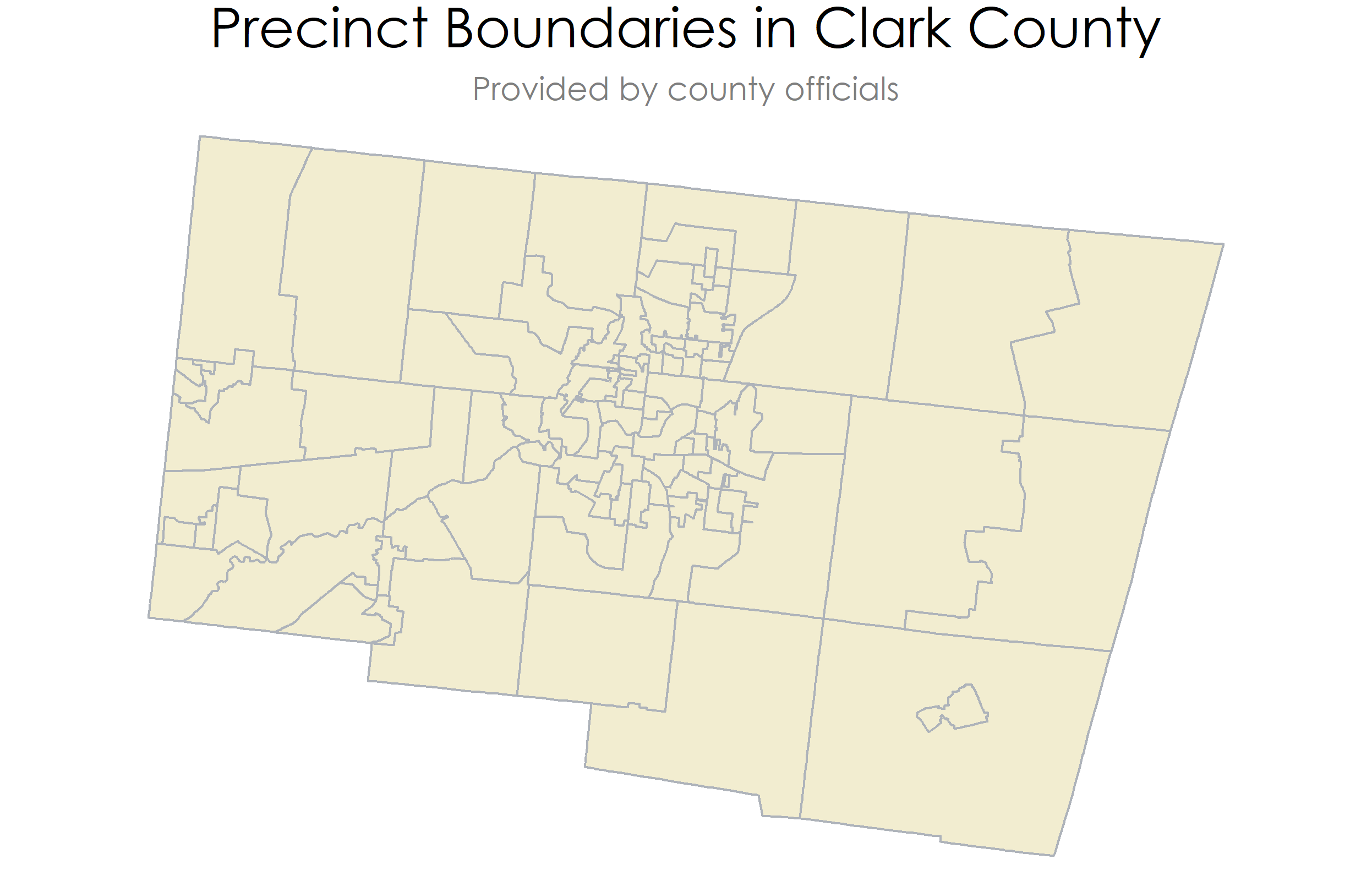
To start, we have the offical shapefile:

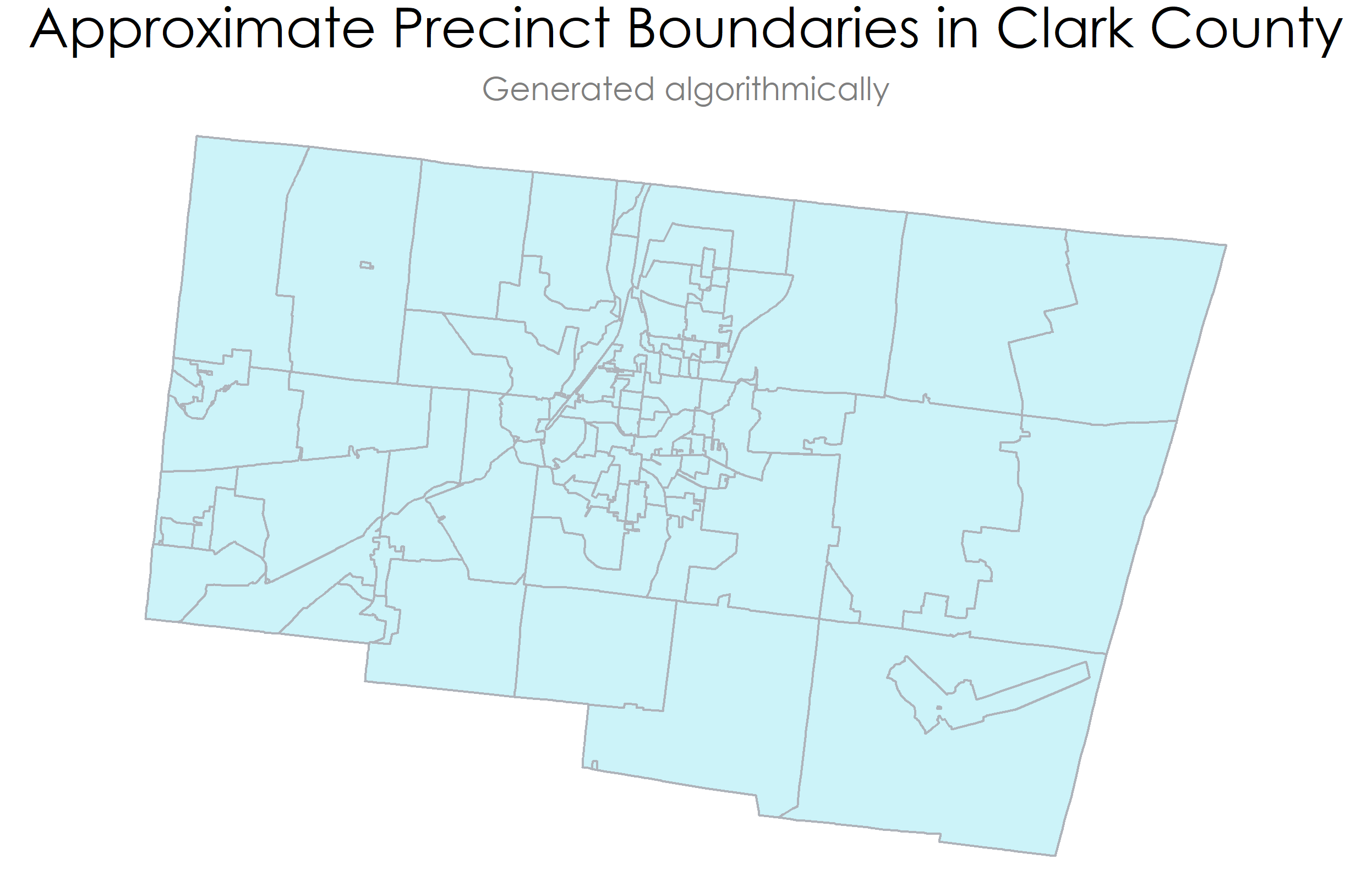
And we have the approximated precincts:

To caluculate the v-measure (as well as corresponding global and local values of (in)homogeneity), we’ll use the {sabre} package in R.

# install.packages("sabre")
library(sabre)
library(sf)

clark_official <- st_read("https://github.com/katiejolly/blog/blob/master/assets/ohio/clark_official.gpkg?raw=true") # geopackage of official precincts
clark_approx <- st_read("https://github.com/katiejolly/blog/blob/master/assets/ohio/clark_approx.gpkg?raw=true") # geopackage of approximated precincts

The basic workflow is load package & load data, use vmeasure_calc(), interpret the results. Functionality for evaluating the degree of spatial agreement with the mapcurves method is also included, but I’m only using v-measure in this post. I’ll often use mapcurves to make sure it gives me a similar value to the v-measure (the function for mapcurves is mapcurves_calc()). For consistency, I usually list the official shapefile as “map1” and the approximated shapefile as “map2.”

vm_clark <- vmeasure_calc(x = clark_official, x_name = PRECINCT, y = clark_approx, y_name = PRECINCT) # x_name and y_name are unique identifiers for the precincts in each of the shapefiles. In these shapefiles they happen to be called the same thing.

vm_clark

## The SABRE results:
##
##  V-measure: 0.95
##  Homogeneity: 0.96
##  Completeness: 0.95
##
##  The spatial objects could be retrieved with:
##  $map1 - the first map
##  $map2 - the second map

The code output tells us the global v-measure, homogeneity, and completeness values. We left the β parameter as the default β = 1. This weights completeness and homogeneity equally. In reality the values are so close that β becomes less important.

We can also get the local values of inhomogeneity for each of the precincts. For example, the regional inhomogeneity values for all 90 precincts in “map1” (the official shapefile) can be retrieved with:

vm_clark$map1$rih

##  [1] 0.036898626 0.057113409 0.001632394 0.010058178 0.029202861
##  [6] 0.005960521 0.050435646 0.007158895 0.039099338 0.052334001
## [11] 0.029467929 0.011739352 0.028959039 0.077805553 0.195526348
## [16] 0.004787040 0.045230763 0.159115164 0.097019248 0.171676805
## [21] 0.131221785 0.149956460 0.049322868 0.189781706 0.096776746
## [26] 0.090179730 0.030527920 0.019714832 0.012197205 0.164626868
## [31] 0.064489187 0.201532963 0.091914643 0.003990779 0.002964396
## [36] 0.002919616 0.130074718 0.066694208 0.208280914 0.136132216
## [41] 0.004568247 0.165028264 0.053723843 0.024823939 0.037866106
## [46] 0.003481937 0.011125713 0.012034109 0.140359525 0.174690711
## [51] 0.024288263 0.091956596 0.052100768 0.015986267 0.055097437
## [56] 0.003442807 0.002601731 0.154708058 0.003480319 0.027410655
## [61] 0.071708507 0.018507759 0.221523420 0.057879958 0.094431642
## [66] 0.036512034 0.014654159 0.028964775 0.071805337 0.077478108
## [71] 0.003459239 0.038919201 0.222934799 0.030306707 0.005732318
## [76] 0.025032241 0.009991034 0.046772304 0.007138603 0.006560449
## [81] 0.016284224 0.019730062 0.060970781 0.336303552 0.034348340
## [86] 0.054703047 0.035584068 0.048018285 0.035154993 0.117438924

Since these values refer to inhomogeneity, we are looking for them to be closer to 0 than 1.

Evaluation and interpretation

We can map the regional inhomogeneity as well to get a better idea of where the approximations are closer to the actual.

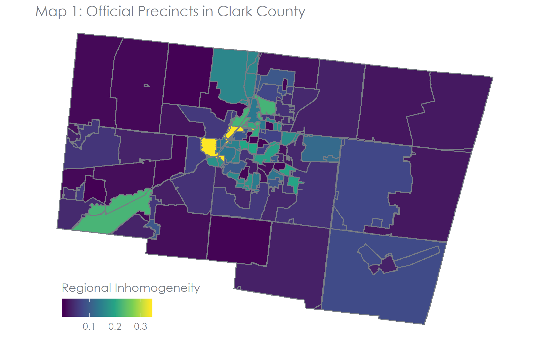
In this map we can see in yellow that the urban (smaller) precincts are not approximated as well as the rural (larger) ones. We could also produce a very similar map from the perspective of the approximated precincts. We think there are a few reasons (that we’ve come up with so far) that we are seeing this particular spatial pattern of the error. First, it’s easier to approximate the precincts in the rural areas with simpler shapes. The urban precincts have much more complex shapes and the nuance can be hard to capture. Additionally, rural precincts seem to be more divided along township lines while urban precincts are more divided along major roads because there are often multiple within a township. We’ve found roads to be difficult to include in the algorithm, but we are looking for ways to improve that now. Overall the errors seem highly clustered (i.e. not randomly distributed) which seems to suggest systemic issues that we could (and should) address in the future.

That’s a quick overview of how we’ve been evaluating our algorithm for precinct approximations. We like the amount of information we can get from v-measure, but are continuously looking for other resources as well. The project in general is a work in progress– feel free to comment if you have ideas or questions! Thanks for reading!