Section 8 Data Wrangling
We will mostly be using the tidyr and dplyr packages for wrangling. With those packages, most wrangling is done with 6 “data verbs.” These are select(), mutate(), filter(), arrange(), group_by(), and summarise(). One quick note: summarise can be spelled the British or American way (as can any word with dual spellings). Much of the software was developed by people in New Zealand, hence the British spellings. I learned with British spellings so that’s what I use, but it works either way.
We can divide our verbs into 3 categories: row verbs, column verbs, and aggregate verbs.
All of the verbs work in a similar way. The general structure is verb(data, action).
8.1 Row verbs
The two row verbs are filter() and arrange(). Filter works by taking out rows that we don’t want in our data. Arrange works by ordering the rows in some way. We will talk about filter first.
8.1.1 Filter
Filter takes in boolean statements and returns only the TRUE ones. For example, >, <, and == are boolean statements. The double equal is R’s way of saying something “is equivalent to.”
Let’s start by creating a dataframe of only Saturday trips.
# create a new dataframe called weekend_trips

saturday_trips <- filter(nice_ride_2018, start_day == "Sat")

dim(saturday_trips) # check that you have these dimensions
## [1] 66778 23We can also make a dataframe of trips that ended after 12 noon.
## [1] 277163 23Let’s say we want some combination of filters. Maybe we want only the Saturday trips that ended after noon? We will use the & operator in between filter actions.
saturday_after_12 <- filter(nice_ride_2018, end_hour > 12 & start_day == "Sat")

dim(saturday_after_12)
## [1] 47806 23Now let’s make a dataframe of all the trips on a weekend day. We will use the | (or) operator in between filter actions.
## [1] 129776 23Let’s add Friday to that list.
weekendFri_trips <- filter(nice_ride_2018, start_day == "Sat" | start_day == "Sun" | start_day == "Fri")

dim(weekendFri_trips)
## [1] 190271 23It gets a little long to write that all out, and this is a pretty simply query. Luckily, R has an %in% operator to filter “in bulk.”
We would get the same results as above by writing:
weekendFri_trips <- filter(nice_ride_2018, start_day %in% c("Sat", "Sun", "Fri"))

dim(weekendFri_trips)
## [1] 190271 238.1.2 Arrange
Arrange is a way to order your dataset by specific variables.
You can order by just one variable, like duration.
8.2 Practice
- How many trips were more than 30 minutes long? This is equivalent to 1800 seconds.
2 (a). How many casual trips were there on Wednesdays, Thursdays, and Fridays?
2 (b) . How many casual trips were there on Wednesdays, Thursdays, and Fridays that were 15 minutes or less?
- How many dockless trips taken by subscribed users were there total?
8.3 Column verbs
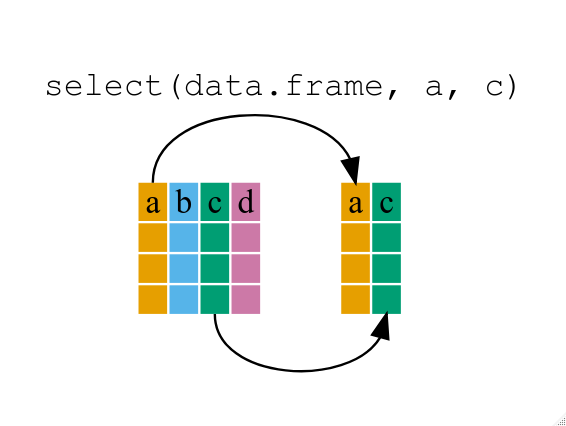
Now that we’ve talked about wrangling the rows, we can think about wrangling the columns. mutate is used to create new columns, while select is used to narrow down the columns you keep in your table.
8.3.1 Mutate
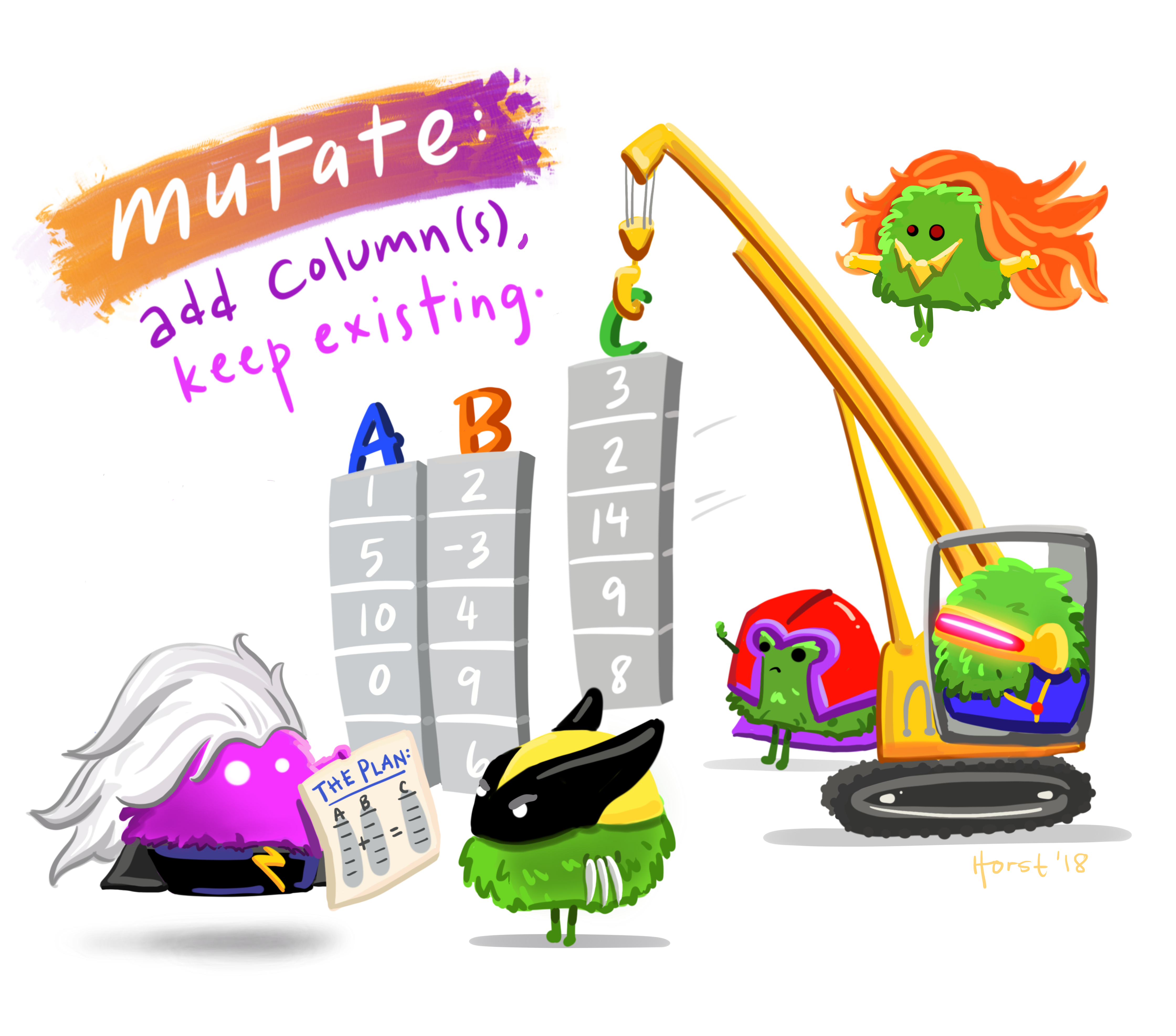
Let’s say we want to create a new duration variable that is in minutes instead of seconds. We can divide our old column by 60 to create the new column.
nice_ride_2018 <- mutate(nice_ride_2018, tripduration_min = tripduration / 60)

head(nice_ride_2018$tripduration_min)
## [1] 22.883333 28.833333 9.116667 14.266667 7.583333 25.9500008.4 Practice
The average trip duration in minutes is 21.257 (see code below).
##    Min. 1st Qu.  Median    Mean 3rd Qu.    Max.
##   1.017   7.200  13.333  21.257  25.400 299.867
Create a new variation called duration_deviation that calculates how far each trip was from the mean. Your resulting column should look something like this…
## # A tibble: 6 x 1
##   duration_deviation
##                <dbl>
## 1               1.63
## 2               7.58
## 3             -12.1
## 4              -6.99
## 5             -13.7
## 6               4.69
8.4.1 Select
8.5 Aggregate verbs
8.5.1 %>%
group_by and summarise are the two main verbs for aggregate statistics, they’re similar to Excel pivot tables. In this section we will also talk about the pipe, %>%, operator. When doing data wrangling tasks there are often many intermediate tables. Maybe you filter, then create a new column, then calculate some summary statistic. Instead of doing all of these as discrete steps, we can link them to push the data through a workflow instead of stopping along the way. This makes life easier for you because you won’t clutter your environment or have to remember what data3 has that data4 doesn’t.
The way it works is fairly straightforward. You use the %>% between data verbs and don’t input a new dataset. The operator is telling your verb to use the previously created data.
For example: if you wanted to filter out just Saturday trips and then convert the duration to minutes, you could do:
saturday <- filter(nice_ride_2018, start_day == "Sat") %>%
  mutate(duration_minutes = tripduration / 60)
Which gives you the exact same output as:
saturday <- filter(nice_ride_2018, start_day == "Sat")
saturday <- mutate(saturday, duration_minutes = tripduration / 60)
With a lot less effort.
8.5.2 group_by & summarise
group_by is how we specify the base unit for aggregate summaries and summarise tells us what to calculate.
We can count the number of trips at each start station. Here we will group by the start station because we want counts per start station. Then to get a count summary we will use the n() function, which counts the number of observations or rows per group.
trips_per_station <- nice_ride_2018 %>%
  group_by(start_station_name) %>%
  summarise(trips = n())

head(trips_per_station)
## # A tibble: 6 x 2
## start_station_name trips
## <chr> <int>
## 1 100 Main Street SE 7604
## 2 10th Street E & Cedar Street 489
## 3 11th Ave S & S 2nd Street 7901
## 4 11th Street & Hennepin 2537
## 5 11th Street & Marquette 2441
## 6 15th Ave SE & Como Ave SE 2807We can also use functions like sum(), mean(), min(), median(), etc. For example, we can calculate the mean trip duration per start station.
mean_duration <- nice_ride_2018 %>%
  group_by(start_station_name) %>%
  summarise(mean_duration = mean(tripduration))

head(mean_duration)
## # A tibble: 6 x 2
## start_station_name mean_duration
## <chr> <dbl>
## 1 100 Main Street SE 1534.
## 2 10th Street E & Cedar Street 982.
## 3 11th Ave S & S 2nd Street 1409.
## 4 11th Street & Hennepin 1158.
## 5 11th Street & Marquette 1675.
## 6 15th Ave SE & Como Ave SE 1018.Then we could also chain a mutate to convert these times to minutes.
mean_duration <- nice_ride_2018 %>%
  group_by(start_station_name) %>%
  summarise(mean_duration = mean(tripduration)) %>%
  mutate(mean_duration_min = mean_duration / 60)

head(mean_duration)
## # A tibble: 6 x 3
## start_station_name mean_duration mean_duration_min
## <chr> <dbl> <dbl>
## 1 100 Main Street SE 1534. 25.6
## 2 10th Street E & Cedar Street 982. 16.4
## 3 11th Ave S & S 2nd Street 1409. 23.5
## 4 11th Street & Hennepin 1158. 19.3
## 5 11th Street & Marquette 1675. 27.9
## 6 15th Ave SE & Como Ave SE 1018. 17.08.6 Practice
- Calculate the number of trips for each user type that occurred at each start station. The structure should look like the example below:
Hint: you can use multiple grouping variables
## # A tibble: 6 x 3
## # Groups:   start_station_name [3]
##   start_station_name           usertype   trips
##   <chr>                        <chr>      <int>
## 1 100 Main Street SE           Customer    6390
## 2 100 Main Street SE           Subscriber  1214
## 3 10th Street E & Cedar Street Customer     188
## 4 10th Street E & Cedar Street Subscriber   301
## 5 11th Ave S & S 2nd Street    Customer    6312
## 6 11th Ave S & S 2nd Street    Subscriber  1589
8.7 Reshaping verbs
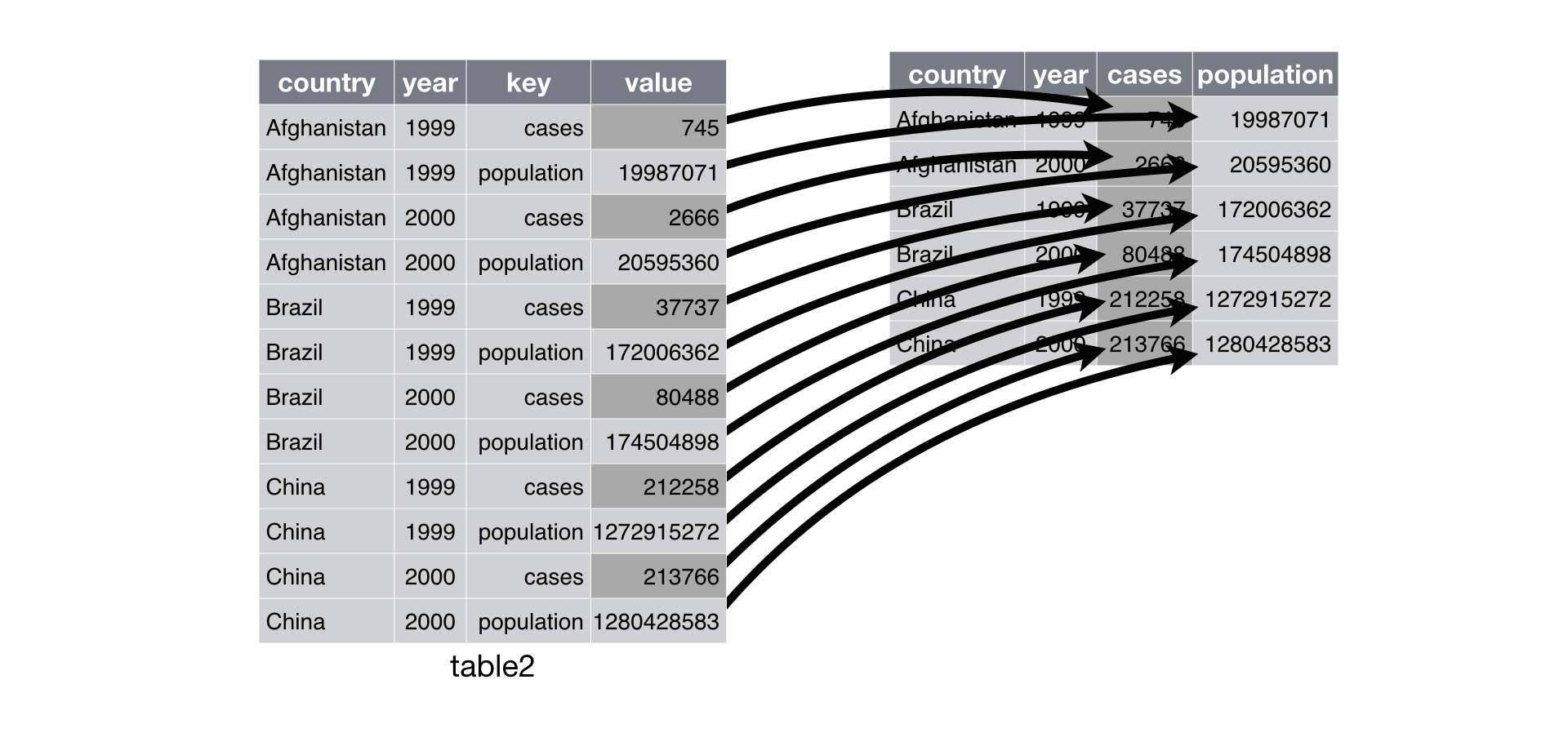
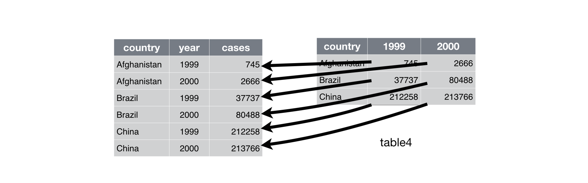
8.7.1 Spread
spread() takes two columns (key & value), and spreads into multiple columns: it makes “long” data wider.
We can spread the data so that we have a column for the number of users of different types at each station. First we can group the data to calculate that number though (your answer from above).
user_types <- nice_ride_2018 %>%
  group_by(start_station_name, usertype) %>%
  summarise(trips = n()) %>%
  spread(key = "usertype", value = "trips")

head(user_types)
## # A tibble: 6 x 3
## # Groups: start_station_name [6]
## start_station_name Customer Subscriber
## <chr> <int> <int>
## 1 100 Main Street SE 6390 1214
## 2 10th Street E & Cedar Street 188 301
## 3 11th Ave S & S 2nd Street 6312 1589
## 4 11th Street & Hennepin 1894 643
## 5 11th Street & Marquette 1907 534
## 6 15th Ave SE & Como Ave SE 1695 11128.7.2 Gather
gather() takes multiple columns, and gathers them into key-value pairs: it makes “wide” data longer.
Let’s say we got the data in the above form (a variable for each user type) and instead want it in a long format. We can use gather() to go the other way.
user_types_long <- user_types %>%
  gather(key = "usertype", value = "trips", 2:3) # specify which columns you want, this reads "1 to 2"

user_types_long
## # A tibble: 410 x 3
## # Groups: start_station_name [205]
## start_station_name usertype trips
## <chr> <chr> <int>
## 1 100 Main Street SE Customer 6390
## 2 10th Street E & Cedar Street Customer 188
## 3 11th Ave S & S 2nd Street Customer 6312
## 4 11th Street & Hennepin Customer 1894
## 5 11th Street & Marquette Customer 1907
## 6 15th Ave SE & Como Ave SE Customer 1695
## 7 15th Ave SE & SE 4th Street Customer 3847
## 8 18th Ave Trail & 2nd Street NE Customer 411
## 9 22nd Ave NE & California Street NE Customer 381
## 10 22nd Ave S & Franklin Ave Customer 1307
## # ... with 400 more rows8.8 Practice
Calculate the number of trips by gender and then spread that dataframe so that you have a column for each of the inputs
Then gather that back to its original format
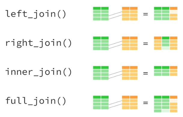
8.9 Joins
dplyr has two different families of joins. First, there’s “joining” joins, which is how we typically think of them
Then there’s also filtering joins.
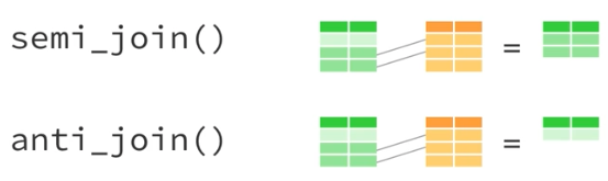
These are useful when you want to filter the rows of one dataset based on another, but you don’t care about the attributes of that second dataset.
The general structure for joins is join(x, y, c("common variable in x" = "common variable in y")). We can join our trips data to the station locations which includes the total number of docks for each station.
First, load the station data.
## # A tibble: 6 x 5
##   number name                           latitude longitude total_docks
##   <chr>  <chr>                             <dbl>     <dbl>       <dbl>
## 1 30000  100 Main Street SE                 45.0     -93.3          27
## 2 30001  25th Street & 33rd Ave S           45.0     -93.2          15
## 3 30002  Riverside Ave & 23rd Ave S         45.0     -93.2          15
## 4 30003  Plymouth Ave N &  N Oliver Ave     45.0     -93.3          15
## 5 30004  11th Street & Hennepin             45.0     -93.3          23
## 6 30005  Hennepin & Central Avenue NE       45.0     -93.3          15
So then if we want to join these by the start_station_name variable in our trips dataset, we would type:
joined <- left_join(nice_ride_2018, station_locations, by = c("start_station_name" = "name"))

glimpse(joined)
## Observations: 409,002
## Variables: 27
## $ tripduration <dbl> 1373, 1730, 547, 856, 455, 1557, 2001,...
## $ start_datetime <dttm> 2018-04-24 16:03:04, 2018-04-24 16:38...
## $ end_datetime <dttm> 2018-04-24 16:25:57, 2018-04-24 17:07...
## $ start_station_id <dbl> 170, 2, 13, 94, 13, 43, 167, 157, 153,...
## $ start_station_name <chr> "Boom Island Park", "100 Main Street S...
## $ start_station_latitude <dbl> 44.99254, 44.98489, 44.98609, 44.97821...
## $ start_station_longitude <dbl> -93.27026, -93.25655, -93.27246, -93.2...
## $ end_station_id <dbl> 2, 13, 94, 13, 43, 167, 157, 153, 201,...
## $ end_station_name <chr> "100 Main Street SE", "North 2nd Stree...
## $ end_station_latitude <dbl> 44.98489, 44.98609, 44.97821, 44.98609...
## $ end_station_longitude <dbl> -93.25655, -93.27246, -93.26023, -93.2...
## $ bikeid <dbl> 2, 2, 2, 2, 2, 2, 2, 2, 2, 2, 2, 2, 2,...
## $ usertype <chr> "Customer", "Customer", "Subscriber", ...
## $ birth_year <dbl> 1969, 1969, 1985, 1985, 1988, 1969, 19...
## $ gender <dbl> 0, 0, 2, 2, 1, 0, 0, 0, 0, 0, 0, 0, 0,...
## $ bike_type <chr> "Classic", "Classic", "Classic", "Clas...
## $ start_month <dbl> 4, 4, 4, 4, 4, 4, 4, 4, 4, 4, 4, 4, 4,...
## $ start_day <ord> Tue, Tue, Tue, Tue, Wed, Fri, Fri, Fri...
## $ end_month <dbl> 4, 4, 4, 4, 4, 4, 4, 4, 4, 4, 4, 4, 4,...
## $ end_day <ord> Tue, Tue, Tue, Tue, Wed, Fri, Fri, Fri...
## $ start_hour <int> 16, 16, 17, 18, 8, 11, 12, 13, 14, 13,...
## $ end_hour <int> 16, 17, 18, 19, 8, 12, 12, 13, 15, 14,...
## $ tripduration_min <dbl> 22.883333, 28.833333, 9.116667, 14.266...
## $ number <chr> "30151", "30000", "30011", "30090", "3...
## $ latitude <dbl> 44.99254, 44.98489, 44.98609, 44.97807...
## $ longitude <dbl> -93.27026, -93.25655, -93.27246, -93.2...
## $ total_docks <dbl> 15, 27, 19, 19, 19, NA, 23, 15, 27, 15...We can see at the end that there’s now a total_docks variable.
8.10 Practice
- Join the trips and stations on the end_station_name variable