Section 9 Visualization, revisited

Now that we have some wrangling experience, we can create some more complex visualizations. This section will be mostly practice questions, promoting active learning and help-finding.

9.1 Facets

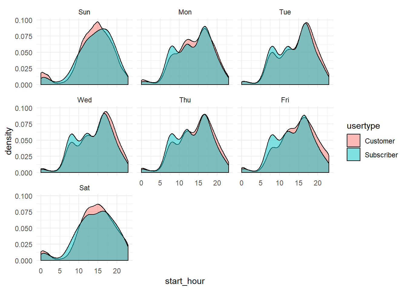
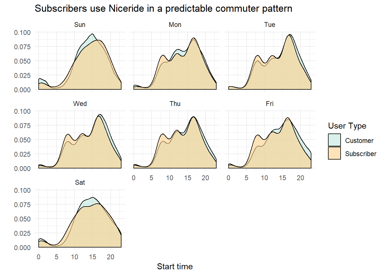
Facets are a way to lay out related plots in a grid. For example, maybe we want to look at hourly patterns by the day of the week.

ggplot(nice_ride_2018, aes(x = start_hour)) +
  geom_density(adjust = 1.5) + # the adjust argument just makes the plots a little smoother
  facet_wrap(~start_day) + # lay out the plots by the weekday
  theme_minimal()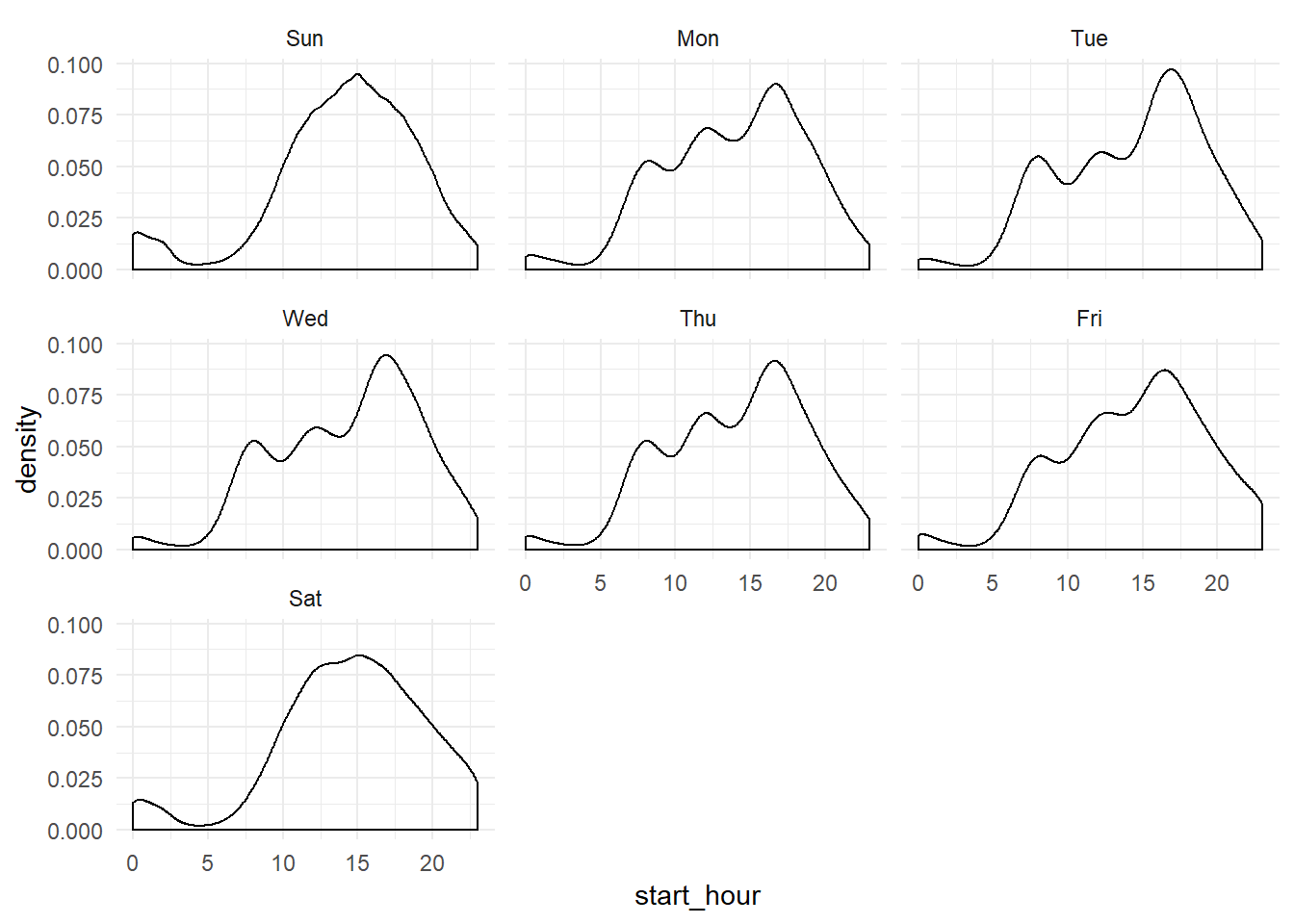

9.2 Multivariate visualization

For two quantitative variables we can use a scatter plot, in ggplot the geom is geom_point(). Another way to summarize these variables would be to use a regression, or geom_smooth(). Non-parameteric regression is that default, but you can also superimpose a linear model.

The ggplot structure is the same, we just now specify both the x and y.

ggplot(nice_ride_2018, aes(x = start_hour, y = tripduration)) +
  geom_smooth() +
  theme_minimal()

## `geom_smooth()` using method = 'gam' and formula 'y ~ s(x, bs = "cs")'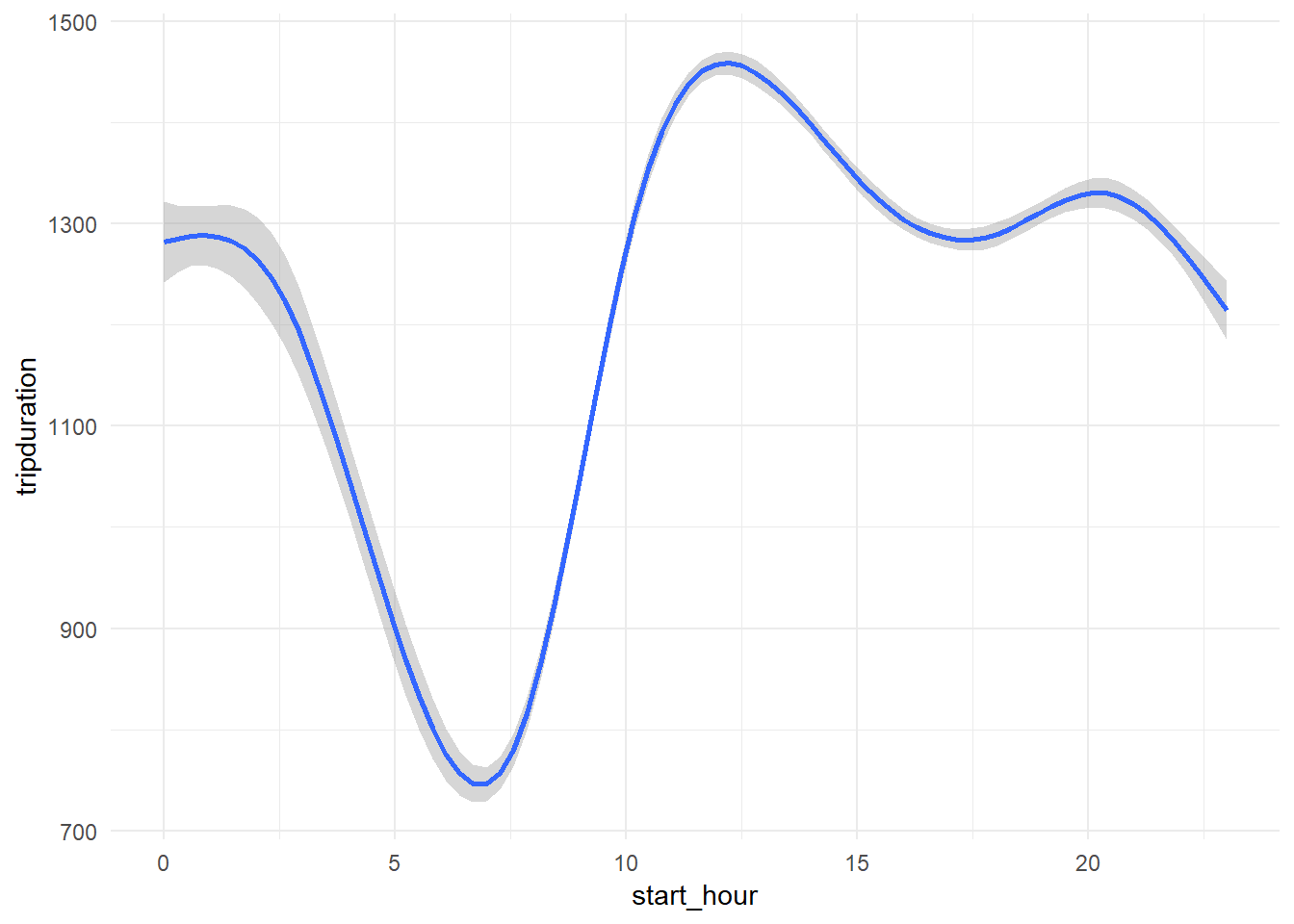

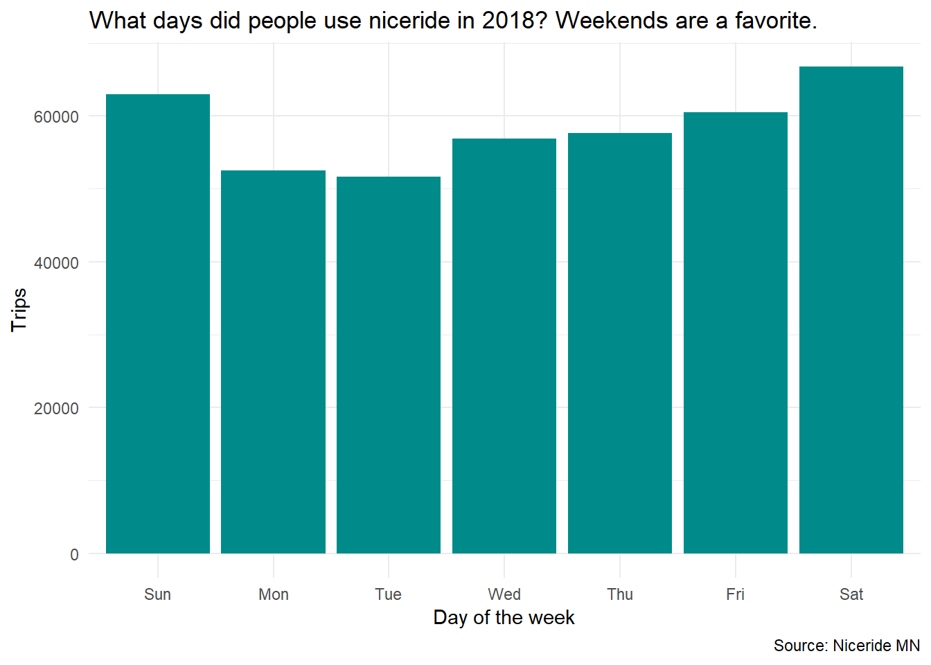
Another multivariate example is one quantitative and one qualitative. A stacked bar chart could be a good way to show this. We will use user type and week day to explain how to make this chart. We will start where we left off in the first visualization section.

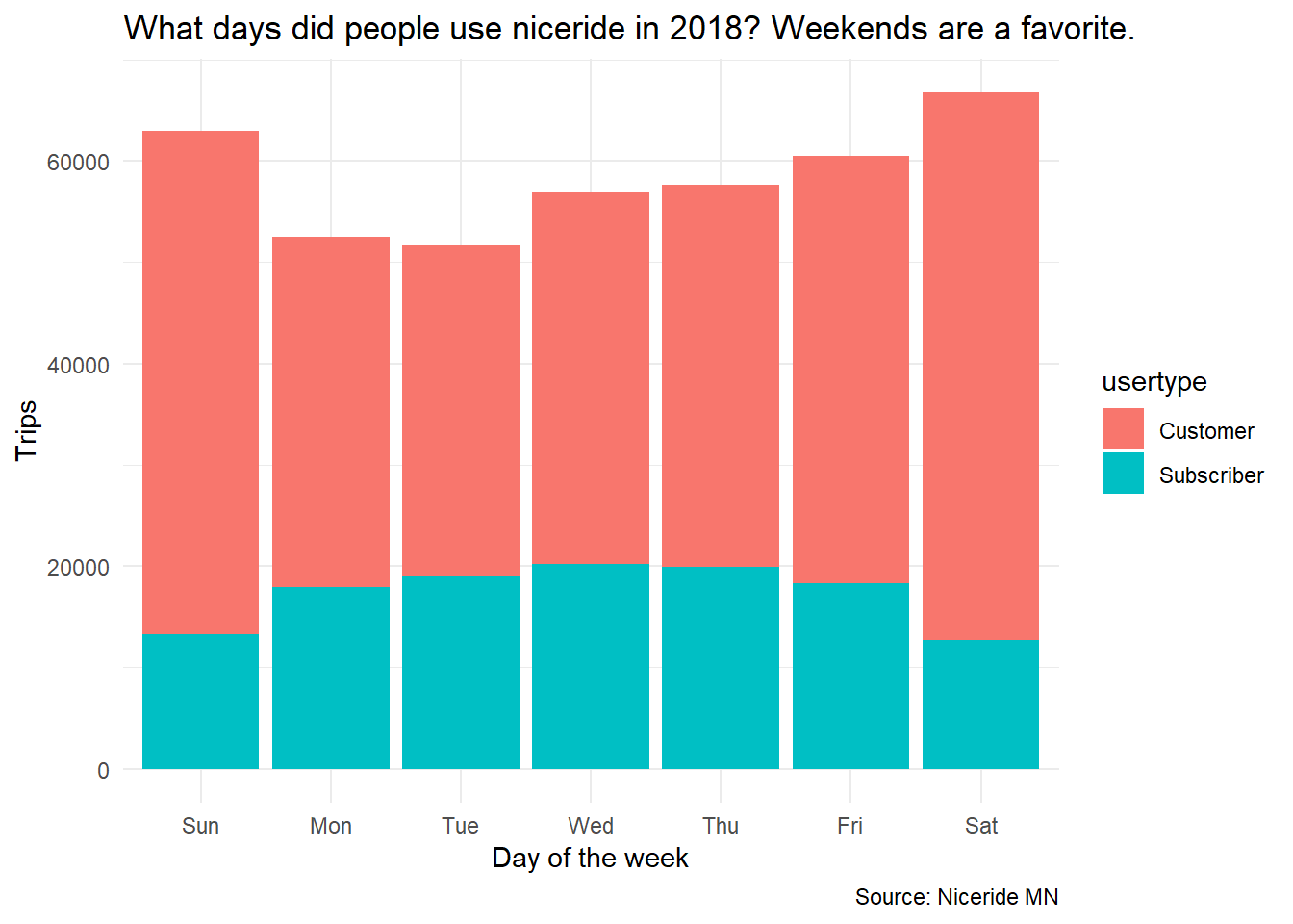
Now, we will create one that differentiates by user type.

First, think about what aesthetic we might be using here. It’s not an axis, but it will map to some other way we can display data.

My hint to you is that you will need to remove fill = ... from the geom_bar() call and think about where else fill might go.

9.3 Practice

• Create a plot of the ten most popular start stations for Classic bikes on Saturdays and Sundays.

Should look like:

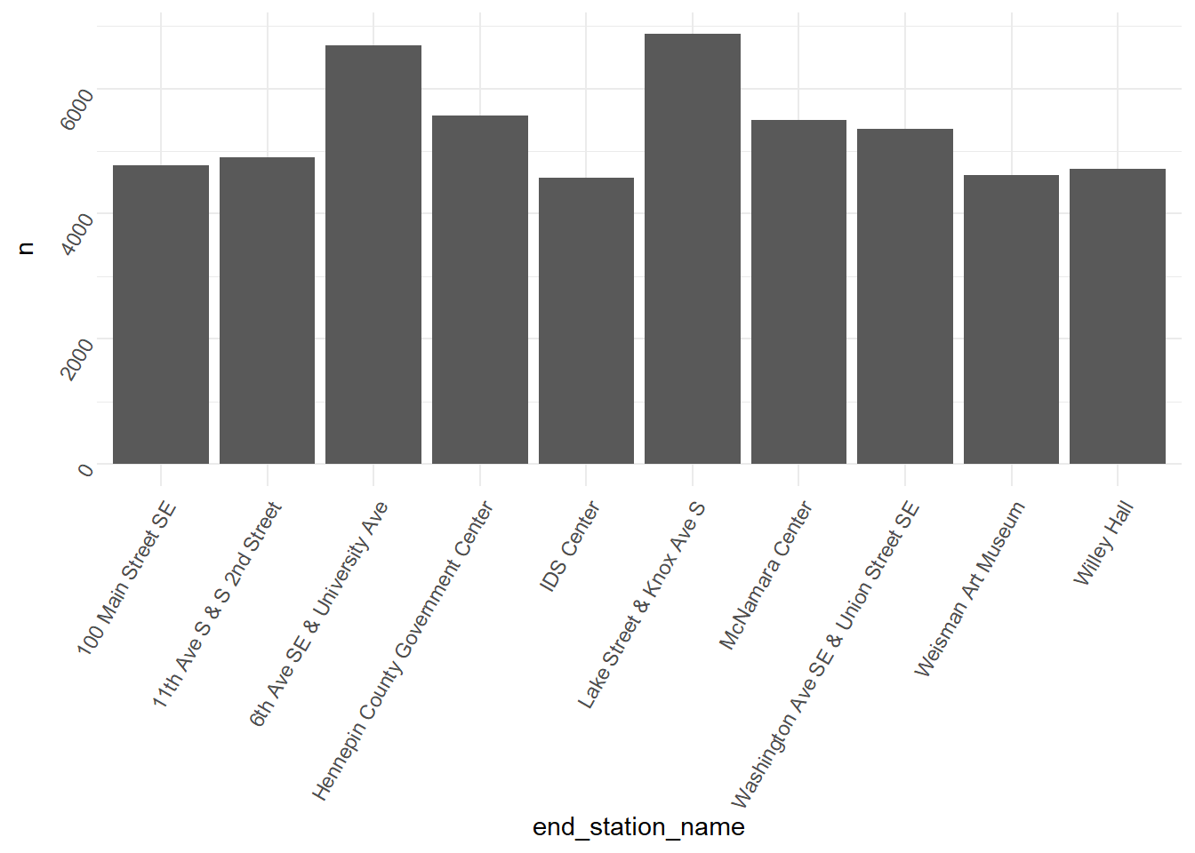
• Create a plot of the ten most popular end stations for Classic bikes on the weekdays.

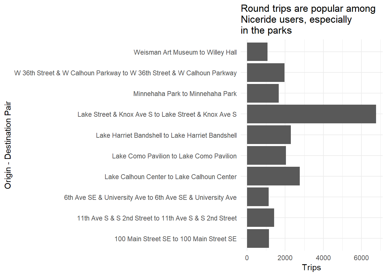
• Create a plot of the 10 most common origin-destination pairs (filter out NULL stations first).

Hints: create a variable of the origin destination pair name with paste(start_station_name, end_station_name, sep = " to ") plus a wrangling verb. Look into coord_flip().

• Create an overlapping density plot of hourly use by user type facetted by weekday (similar to above).

• Then change the colors on that plot

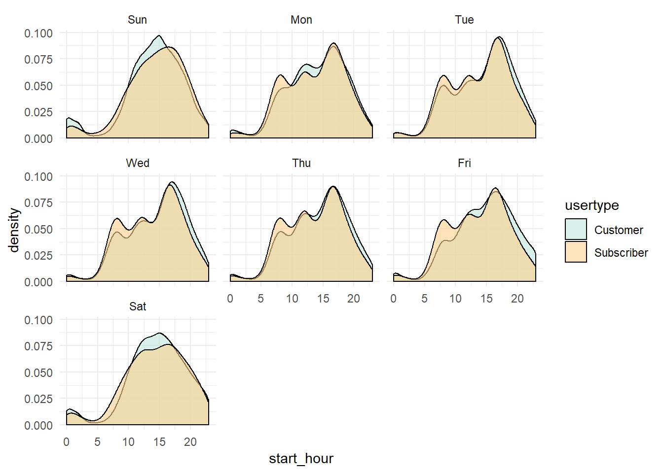
• And add better labels, including a legend title (read the help doc from above).

• On a new plot, make a “map” using the longitude and latitude variables as a scatter plot